SLOs from Mesh Metrics: A 30-Day Implementation Playbook

If you run Kubernetes in production, you’ve probably heard the term Service Level Objective (SLO) in countless planning meetings over the last 2 years. But have you ever defined one? When I have, it was on a gut feeling: I never had a metric I trusted enough to defend when the page went off at 2 am, and the thresholds were never really agreed on. The great news is, if your services are meshed, you already have the metrics. 

This is a hands-on playbook. You’ll learn which five SLOs to define first for east-west service traffic and how Linkerd’s golden metrics map to each one. You’ll get the exact PromQL (the Prometheus query language) for every one of them, how to alert on them without paging yourself into oblivion, and the order to roll it all out over your first month. 

Everything here was run on a live single-node K3s v1.34.6 cluster with Linkerd edge-26.6.3, the OpenTelemetry Demo as the workload, and a bring-your-own Prometheus and Grafana. Every query and every number below came off that cluster.

What an SLO actually is (and isn’t)

Let’s start with a Service Level Indicator (SLI). An SLI is a number that measures one service health dimension, like the fraction of requests that succeed. A Service Level Objective (SLO) is a target for that number over a window, like 99.9% success over 30 days. A Service Level Agreement (SLA) is an SLO with financial penalties attached to it, like a cloud provider owing you service credits when monthly uptime drops below 99.9%.

The job of an SLO is narrow: it gives the on-call engineer a number to defend and a threshold to page on. That’s it. It is not a dashboard with every metric you have, and it is not an aspiration to 100%. An SLO you can’t measure is a wish, and an SLO you set to 100% is a pager that never sleeps.

Where the metric comes from

The reason my team struggled to define an SLO was the practical wall right behind the concept. We wanted to track availability, but we didn’t have a metric for it. Instrumenting every service to emit a clean success-rate counter is a project no one is looking forward to.

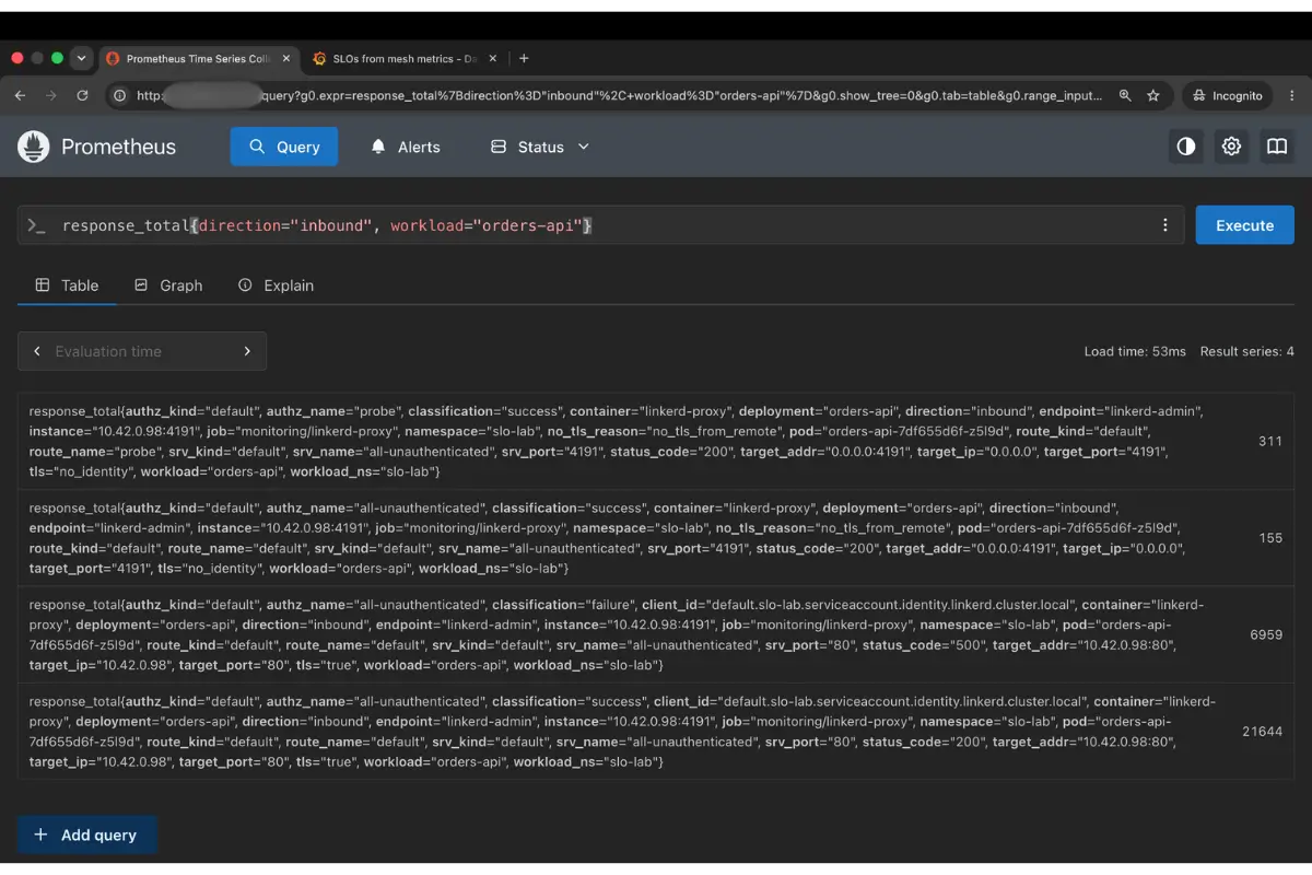
Meshing removes that work for east-west traffic. The moment a workload is meshed, its Linkerd microproxy starts recording every request it handles, and 2 metrics carry everything the SLOs need:

• response_total, a counter of responses with a classification label of success or failure, which gives you request rate and error rate.
• response_latency_ms_bucket, a latency histogram, which gives you p50, p95, and p99.

‍

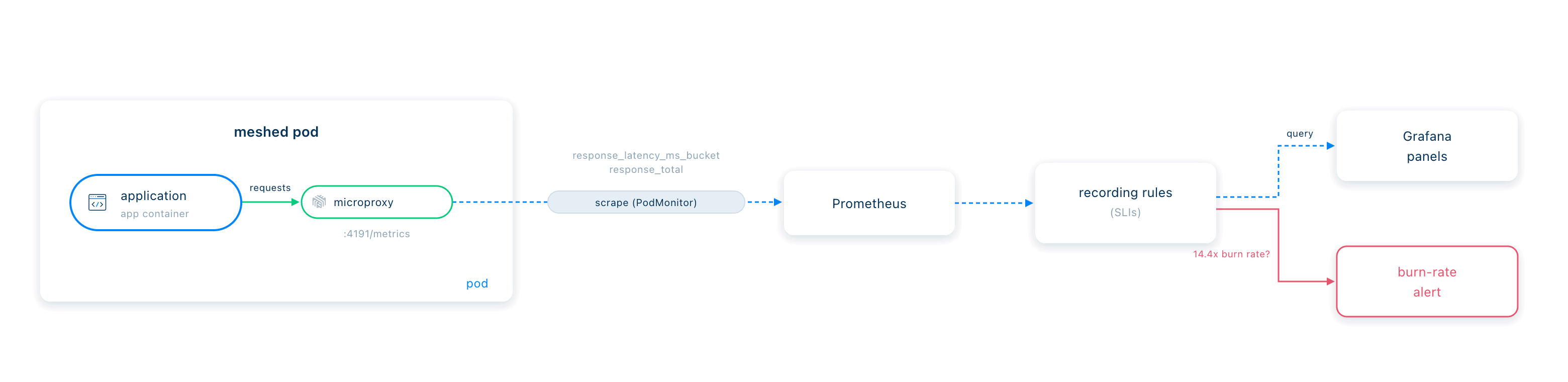
Here’s a single inbound response_total series from orders-api on the live cluster, with a few labels trimmed for readability:

response_total{
  workload="orders-api", namespace="slo-lab", direction="inbound",
  classification="failure", status_code="500", tls="true",
  srv_name="all-unauthenticated", target_port="80"
}

Two things to keep in mind: The tls="true" is mutual TLS between meshed pods, which you get for free. Meanwhile classification="failure", backed by the status_code="500", is the load-bearing label: the proxy already decided this was a failed request, so your availability SLI is one division away, and the collection already happened.

There’s a second benefit, but less obvious than the dashboard. A number you trust changes the conversations you have. When you can point at a real success rate, you can defend a rollback in a review, push back on a latency target nobody actually measured, and make the case for reliability work with data instead of a hunch. The metric is the argument.

If you want a full overview of what mesh-derived metrics do and don’t cover versus your application’s own telemetry, take a look at my earlier post, OTel and mesh-derived metrics. This post takes the metrics as given and turns them into SLOs.

The 5 SLOs to ship first

Five SLOs cover the questions an on-call engineer asks. For each one, we cover what it measures, the exact PromQL, a starting threshold, and why that threshold. Every query groups by a workload label that we relabel onto the proxy metrics, so it covers every meshed service with no per-service configuration.

A rule from the Google SRE Workbook applies to every threshold below: Don’t pick a number off a chart. Read your current baseline, set the target just under it, and tighten over time. The mesh is already collecting that baseline for you.

1. Availability

Availability is the fraction of inbound requests a service handles successfully:

sum by (workload) (rate(response_total{direction="inbound", classification="success", target_port!="4191"}[5m]))
/
sum by (workload) (rate(response_total{direction="inbound", target_port!="4191"}[5m]))

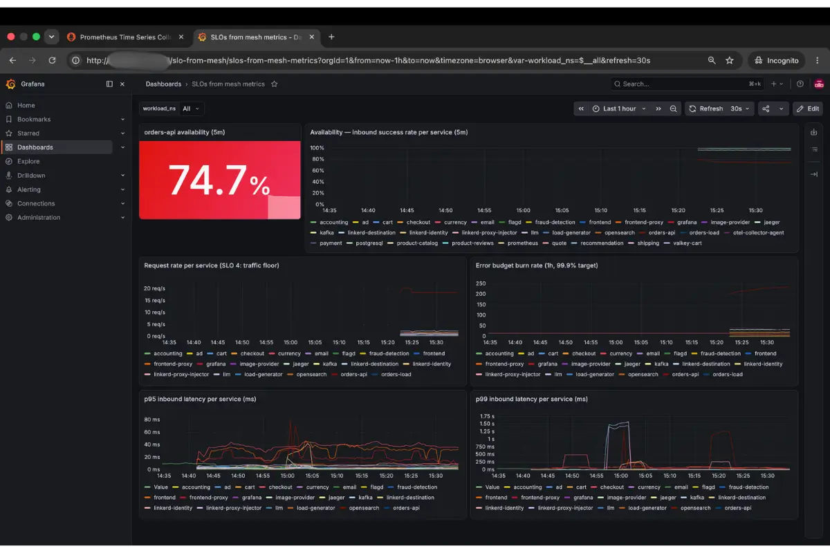
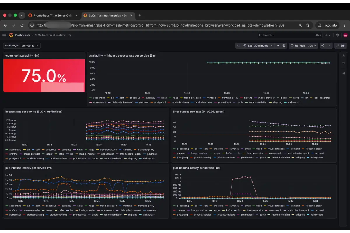
Start at 99.9%, which buys a 43-minute error budget per month. The ladder makes the choice concrete: 99% is 7.2 hours a month, loose enough that a real regression hides inside it; 99.99% is 4.3 minutes a month, which, in my experience, usually needs redundancy internal services don’t have yet. 99.9% is the one I start at, then tighten once I’ve watched a service sit above it. On this cluster the healthy demo services run at essentially 100%, so 99.9% is achievable, which is the test a starting SLO has to pass.

2 and 3. p95 and p99 latency

The latency SLOs come as a pair: p95 is the latency a typical request sees, and p99 is the tail, the slowest 1 in 100 requests.

histogram_quantile(0.95, sum by (workload, le) (rate(response_latency_ms_bucket{direction="inbound", target_port!="4191"}[5m])))

Swap 0.95 for 0.99 for the p99 SLO. There is no universal latency threshold, and this cluster proves why: p95 ranges from 1 ms on postgresql to 39 ms on frontend, and p99 on checkout reaches 75 ms. A blanket “500 ms p95” target would be meaningless for a service that normally answers in 2 ms. Read the current distribution off the panel, then set the target at a round number a little above today’s value. You need both: p95 is what a typical request sees. p99 is the tail, and it can be slow while p95 looks fine, so a p95 target alone hides a bad p99.

A caveat for the reader who checks: response_latency_ms_bucket uses coarse exponential buckets, so a p99 of 75 ms is interpolated from bucket boundaries and is only accurate to within a bucket. That’s fine for an SLO. Just know it before someone argues about the second digit.

4. Request-rate floor

The request-rate floor answers a different question: Is the service receiving traffic at all?

sum by (workload) (rate(response_total{direction="inbound", target_port!="4191"}[5m]))

This is an example of what’s often referred to as “the dead man’s switch.” An availability SLO reads a perfect 100% when traffic drops to zero, because no requests mean no failures, and a silent upstream break looks identical to “healthy but quiet.” The request-rate floor, SLO number 4, catches the difference.

The floor has no number you can copy, and unlike the others, it belongs only on services that are supposed to have steady traffic. Set it relative to the service’s own normal load, for example, alert when the 5-minute rate falls below 20% of what it was serving 15 minutes ago. Don’t put a floor on a naturally bursty, low-traffic service if you want to avoid lots of unnecessary pager alerts.

The first version of this query showed traffic that was not there, and the reason matters. After I cut all traffic to a test service, its request rate stalled at about 0.3 rps instead of falling to zero. That residual was entirely kubelet liveness and readiness probes hitting the proxy’s admin port, target_port="4191", which the proxy dutifully counts as response_total. Those always-200 probes do 2 bad things: they slightly inflate every availability number by padding the success count, and they put a permanent noise floor under every service so a real outage never reads zero. That’s why every query in this post excludes target_port="4191". It’s the same class of probe pollution I’ve flagged before in the RED vs USE guide, and you only have to learn it once: the mesh measures everything, including the health checks, so you filter the admin port out before you trust the number.

5. Error-budget burn rate

The last SLO measures how fast you’re spending the budget, which is what tells you whether today is a good day to ship a risky change.

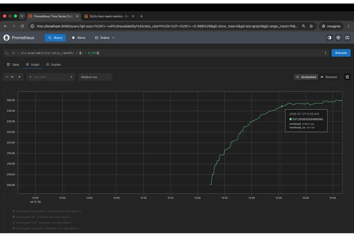
(1 - sli:availability:ratio_rate1h) / (1 - 0.999)

A burn rate of 1 spends the entire 30-day budget in exactly 30 days. On this cluster, the degraded orders-api burns at about 234x, still climbing as the 1-hour window ages out its healthy past: a service dropping roughly 1 in 4 requests annihilates a 99.9% budget almost immediately. The alerting section sets the page threshold at 14.4x. You’ll see in the next section why the burn rate is the number you alert on and why the raw success rate makes a noisy alert.

Going per-route

Everything above is per-service, which is where you start. When a service breaches its latency SLO but serves several endpoints, the per-service number can’t tell you which one is at fault. Attach a Gateway API HTTPRoute to the service and Linkerd emits per-route counters on outbound_http_route_request_statuses_total, labeled by route_name. I split the frontend service into named routes and got clean per-route rates:

outbound_http_route_request_statuses_total{parent_name="frontend"} by route_name:
  frontend-products   0.41 rps
  frontend-cart       0.22 rps
  frontend-checkout   0.06 rps

(There’s also an older route_response_total metric driven by ServiceProfile route definitions. If you’re already using ServiceProfiles, that path still works. New setups should reach for HTTPRoute.)

All six panels behind these queries ship as one importable Grafana dashboard. The JSON is in the companion repo. Point any Grafana at your Prometheus, import the file, and every panel above populates.

Alerting that doesn’t fire on every deploy

A common mistake is to alert directly on the SLO breach.

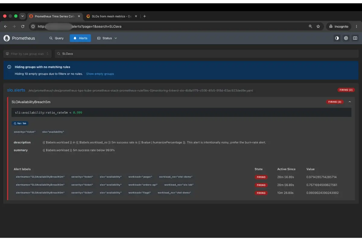
sli:availability:ratio_rate5m < 0.999

This alert fires on the next deploy, the one after that, and every transient blip in between, because the SLI is computed over a 5-minute window. Within a week your team has an inbox rule for it, and now you have an expensive metric nobody looks at.

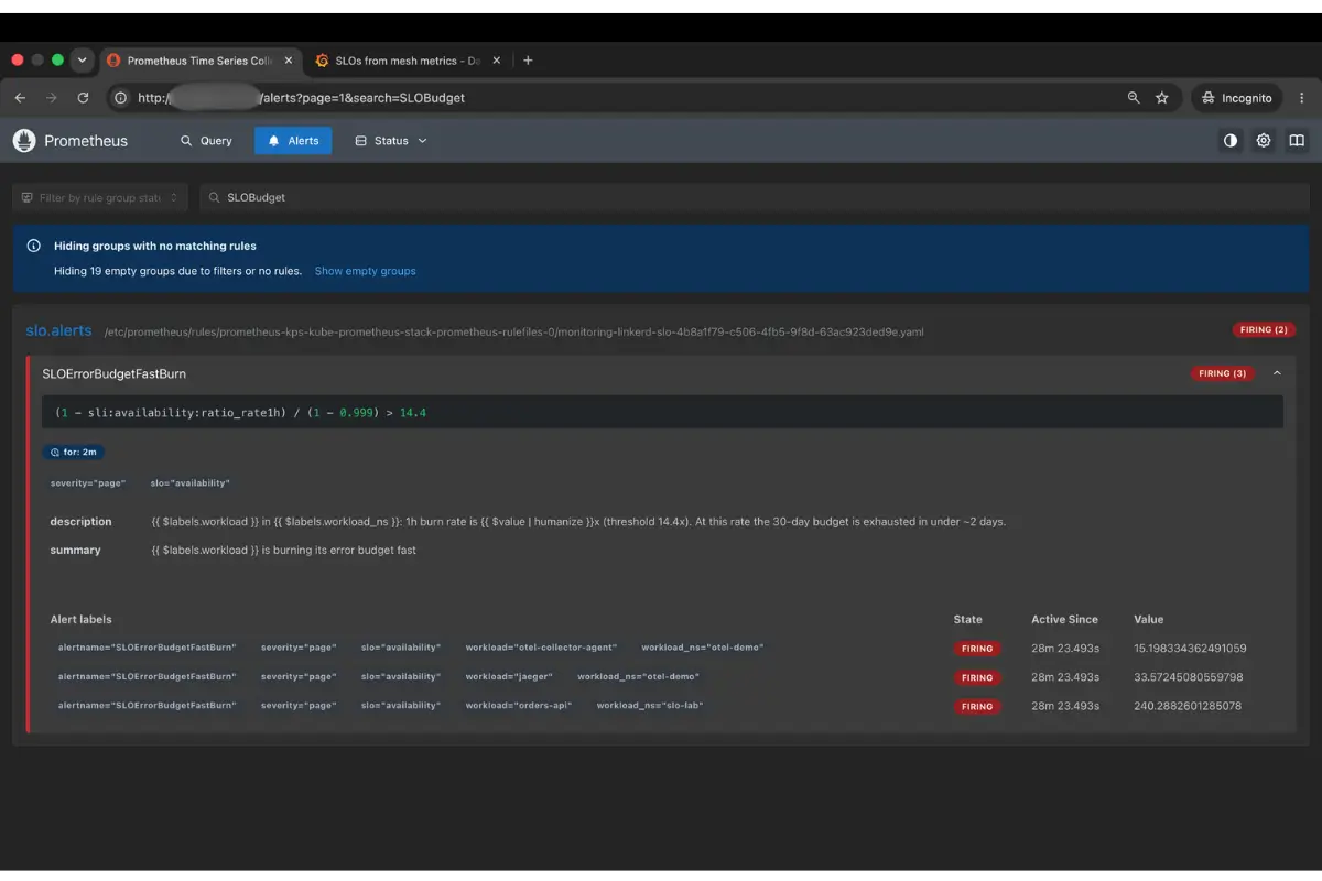
Alert on the burn rate instead. The question that really matters is whether you’re spending the budget fast enough to care about. The Google SRE Workbook’s fast-burn threshold is 14.4x over one hour, and the number comes straight from the budget arithmetic: over a 30-day (720-hour) budget, a burn rate of 14.4 spends 2% of the entire month’s budget in a single hour, so if it holds, the budget is gone in about two days, and that is worth a page, while a brief dip during a single deploy is not.

- alert: SLOErrorBudgetFastBurn  expr: (1 - sli:availability:ratio_rate1h) / (1 - 0.999) > 14.4  for: 2m  labels:    severity: page  annotations:    summary: "{{ $labels.workload }} is burning its error budget fast"

This is shipped as a Prometheus Operator PrometheusRule, which is how you deliver alerting rules when you’re running kube-prometheus-stack. Side by side on the same breach, the comparison settles it: the naive < 99.9% rule and the burn-rate rule both fire for the genuinely broken orders-api, but only the naive one would have fired for every healthy service that dipped for a minute during a rollout. Ship the burn-rate one, and your on-call rotation stays sane.

There is one limitation I’d like to point out because it actually happens: A single-window alert. Production setups usually add a slower second window, say 3x over 6 hours, to catch a slow leak that the 1-hour window sleeps through. That’s multi-window, multi-burn-rate alerting, and it’s a post of its own. The single fast-burn window is the right place to start.

The 30-day rollout

You don’t roll this out all at once, because each service needs its threshold read from its own baseline, and you don’t alert on day one, because paging on a metric you don’t trust yet teaches the team to ignore it. Here’s the pacing I recommend, as an order to follow rather than a deadline to hit.

• In week 1, mesh one service and watch availability only. Confirm response_total is flowing into your Prometheus, write the success-rate query, and watch it for a few days. The goal is to trust the metric before you page on it.
• In week 2, add the p95 and p99 latency SLOs to that same service. Read the real distribution and set thresholds from it, still with no paging.
• In week 3, roll out to the rest of the namespace. Your scrape config already collects every meshed pod, so this is mostly meshing the remaining workloads and setting each one’s thresholds from its own baseline. Resist the urge to pick one global number.
• In week 4, turn on burn-rate alerting and hold the first error-budget review. Add the recording rules and the fast-burn alert, then ask the question the whole program exists to answer: did anything burn, and can we afford the next risky deploy?

The order matters. First you need the metric, then thresholds, then breadth, and then alerting. Teams that alert in week 1 have trained themselves to ignore the alerts by week 2.

Where each one earns its place

An SLO is only as good as the metric under it, and mesh-derived metrics are trustworthy for east-west traffic for a specific reason: the proxy is the authoritative observer. It sits in the request path for every meshed call, so it counts what actually happened on the wire, with mTLS identity attached, rather than what an application library decided to report. You get an SLO program for every meshed service without instrumenting a single one of them.

This comes with a prerequisite. It covers meshed workloads only, because an unmeshed pod emits no response_total and so has no SLO. Meshing the workload is step 0, and it’s the step that makes every step after it free.

The playbook also stops at a boundary. These are request SLOs: the RED view of traffic, its rate, errors, and duration. They say nothing about resource saturation, the USE view (utilization, saturation, errors) of whether a node or container is running out of CPU, memory, or file descriptors. That half comes from node and container metrics, and Brendan Gregg’s USE method is the canonical treatment. I put both side by side in the RED vs USE guide if you want the resource half, too.

About the Author

Mesut is a DevOps engineer, CNCF TAG Infrastructure Tech Lead and an OSS contributor, based in Stuttgart, Germany. You can find his work on GitHub and connect with him on LinkedIn. 

FAQ

Do I need to instrument my application code to define Kubernetes SLOs with a service mesh?

No, you do not need to instrument your application code. By using a service mesh like Linkerd, the proxy automatically captures request metrics, including latency and success rates, directly from the network. This eliminates the need to modify your code to emit custom telemetry.

Can I define SLOs using mesh metrics for services that are not part of the service mesh?

No. You cannot define SLOs using this method for unmeshed services because they do not emit the required proxy metrics. Only workloads running with a service mesh sidecar provide the granular traffic data, such as response totals and latency histograms, necessary for these SLO pipelines.

Are these service mesh SLOs compatible with both gRPC and HTTP traffic?

Yes. Linkerd mesh metrics capture and classify traffic for both gRPC and HTTP protocols. The proxy successfully identifies and handles status codes for both, allowing you to accurately calculate success and error rates without requiring protocol-specific configuration.

Why must I exclude target_port="4191" when querying SLO metrics?

You must exclude target_port="4191" because this is the Linkerd proxy’s admin port, which receives kubelet health-check probes. These probes always return a 200 OK status. If included in your queries, they artificially inflate your success rate and create a "noise floor," effectively masking real traffic drops or outages.

Sources

• Google SRE Workbook, Implementing SLOs and Alerting on SLOs
• Brendan Gregg, the USE method
• Linkerd proxy metrics reference
• Prometheus alerting rules documentation

‍